I’ve been talking to Iain, MM0ROR a bit on the radio. After I persuaded him to build a 70cm version of the 1/4 wave vertical antenna I built earlier this year, I helped him test it on the radio tonight from my new /m setup.

Initially I drove to the picturesque Aberdeen Beach, then the less pretty 57North Hacklab, and finally I took the long road to the very lovely Balmedie Beach, and for the bulk of the drive nattered away to Iain about nonsense and radios.

It’s the first time we’ve easily managed simplex, 70cm for an extended period of time, and it was awfully enjoyable. His new antenna outperforms the existing 2m/70cm one, hopefully this means the ScotCon Monday night Nets become more viable.

In the back of my head, I remembered using Splat to model radio coverage - I figured I’d try it for the route.

Splat

Splat describes itself as An RF Signal Propagation, Loss, And Terrain analysis tool. It’s packaged for debian, and lives on the command line.

At first glance, it’s a little unfriendly, but this pdf is a comprehensive, easy to access guide! Better yet, it’s just the man page but in a pdf. You can apt install splat, man splat and read all this handy-dandy data.

Splat needs a few things to give you line of sight/point to point reports and coverage reports.

Topographical Data

It needs location data fed in. This must be topographical location data - the man page’s recommended source is the data from the Space Shuttle STS-99 Radar Topography mission, which is a 1 degree by 1 degree radar, topographical map of the world (How cool is that?!).

This can be downloaded from here - I needed an account. The higher resolution files referenced in the man page aren’t available for outside the US & its territories, so we’re stuck on SD, not HD.

Once this was downloaded it, I coped it into my folder structure, ~/Dev/Radio/splat/downloads, unzipped it and ran the srtm2sdf tool included with splat on the resultant files. This output the maps into a format splat can understand. I copy the resultant .sdf files to ~/Dev/Radio/splat/sdf for convenience.

Station Location Data

Now splat knows the hills, it needs to know where you live. There are two files to describe this - first, the pleasingly named .qth file, contains your latitude, longitude and antenna height above sea level. Secondly, the .lrp file details the working conditions. Frequency, polarisation, ERP, etc.

This drives the bulk of the simulation. I keep my qth and lrp files in a folder for the study, as all output will go there also.

For my mobile location:

hibby@fennec ~/D/R/s/study> cat mm3zrz-m.qth
MM3ZRZ-M
57.253760077
2.0429511661
13m

hibby@fennec ~/D/R/s/study> cat mm3zrz-m.lrp
15.000  ;Earth Dielectric Constant (Relative permittivity)
0.005   ;Earth Conductivity (Siemens per meter)
301.000 ; Atmospheric Bending Constant (N-units)
433.550 ; Frequency in MHz (20 MHz to 20 GHz)
6	;Radio Climate (5 = Continental Temperate)
1	;Polarization (0 = Horizontal, 1 = Vertical)
0.50	;Fraction of situations (50% of locations)
0.90	;Fraction of time (90% of the time)
10	; Effective Radiated Power (ERP) in Watts (optional)

There was a corresponding one for MM0ROR with his ~30W or so I assumed he was TXing at. Naturally, as a good friend, I’m not revealing his location on the internet.

Point to Point study

From Iain to me, the command was pretty simple:

splat -t mm0ror.qth -r mm3zrz-m.qth -d ../sdf -p profile.png

He is the Transmitter (-t), I am the Receiver (-r), my topo maps are in ../sdf, output a profile.png showing elevation.

I get a text file called MM0ROR-to-MM3ZRZ-M.txt, which has an interesting analysis of the link - i see distances, azimuth angle, elevation angle for both sites, and then this really fascinating summary:

Summary For The Link Between MM0ROR and MM3ZRZ-M:

Free space path loss: 106.92 dB
ITWOM Version 3.0 path loss: 120.20 dB
Attenuation due to terrain shielding: 13.28 dB
Field strength at MM3ZRZ-M: 57.38 dBuV/meter
Signal power level at MM3ZRZ-M: -72.62 dBm
Signal power density at MM3ZRZ-M: -88.41 dBW per square meter
Voltage across a 50 ohm dipole at MM3ZRZ-M: 66.88 uV (36.51 dBuV)
Voltage across a 75 ohm dipole at MM3ZRZ-M: 81.91 uV (38.27 dBuV)
Mode of propagation: Line of Sight
ITWOM error number: 0 (No error)

As splat has no information about the receiving antenna, it gives some advice.

The profile looks like:

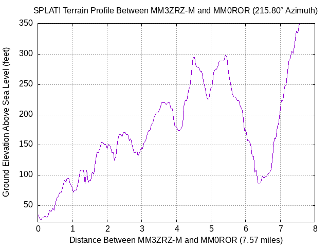
It’s pretty cool, eh? I get that it’s maybe aimed more at microwave line of sight stuff that I use Pathloss for in a professional context, but it’s fun to be able to do it at home too. There’s helpful advice to do with moving antennas to ensure integrity of Fresnel zones, that’s helpful for antenna placement!

Link Profiling

The above link is for the 70cm band - 433.550MHz.

We attempted a 2m band contact, and this didn’t work. There are a number of reasons for this (Iain’s qth doesn’t have a great antenna, etc), but I figured I’d run the calculation at 145.550 MHz:

Free space path loss: 97.44 dB
ITWOM Version 3.0 path loss: 109.12 dB
Attenuation due to terrain shielding: 11.68 dB
Field strength at MM3ZRZ-M: 58.98 dBuV/meter
Signal power level at MM3ZRZ-M: -61.54 dBm
Signal power density at MM3ZRZ-M: -86.81 dBW per square meter
Voltage across a 50 ohm dipole at MM3ZRZ-M: 239.49 uV (47.59 dBuV)
Voltage across a 75 ohm dipole at MM3ZRZ-M: 293.31 uV (49.35 dBuV)
Mode of propagation: Line of Sight
ITWOM error number: 0 (No error)

What we see on 2m is a ~9dB Lower Free Space Path loss, as expected, and ~2dB lower attenuation due to terrain shielding.

This ~11dB difference is clearly reflected in the received signal power level, which is approximately 11dBm higher for 2m band, and for the dipole voltages - both ~11dBuV larger.

I was expecting 70cm to diffract more, maybe I need to do some more reading… and Iain definitely needs better antenna placement!

Coverage Study

Splat also lets me study what the predicted coverage for my radio would be from that location, combining the topographical information with what it can guess about my antenna (10W ERP, 11m ASL is all I told it)

splat -t mm3zrz-m.qth -d ../sdf -c 20 -m 1.333 -o map-car.ppm

This has the new flags of -c 20, setting all receive antennas at 20' above ground level, and -m 1.333, which tells splat to use what’s known as the “four-thirds earth” model, a common modelling mode for line of sight systems.

This outputs this image:

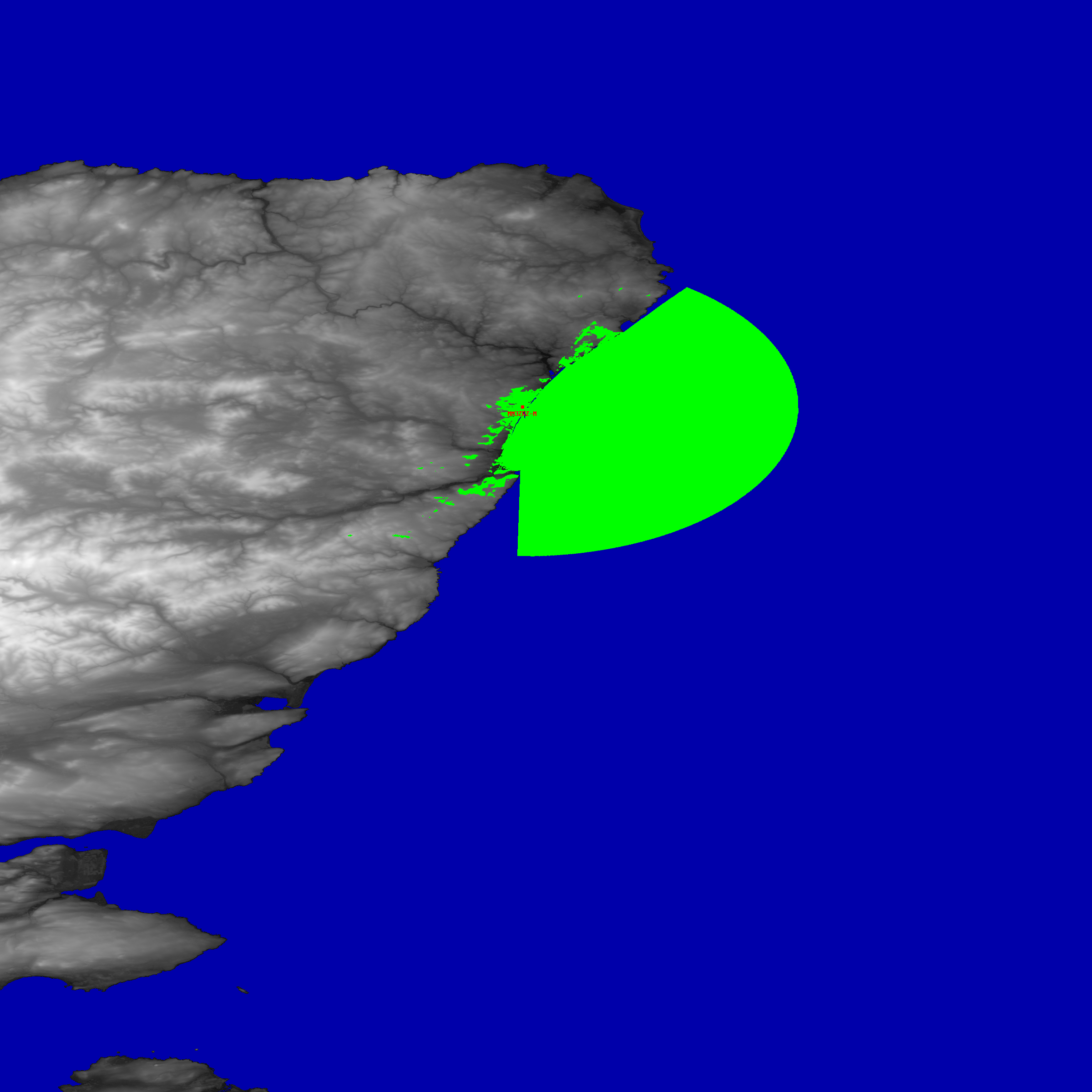
It’s clear I don’t have the best coverage, but areas with raised antennas around the city, and all of the local sea will be able to hear me!

Covering all my friends

Okay so, I can repeat this for multiple stations. Let’s add Iain (with an obfuscated location) to the mix:

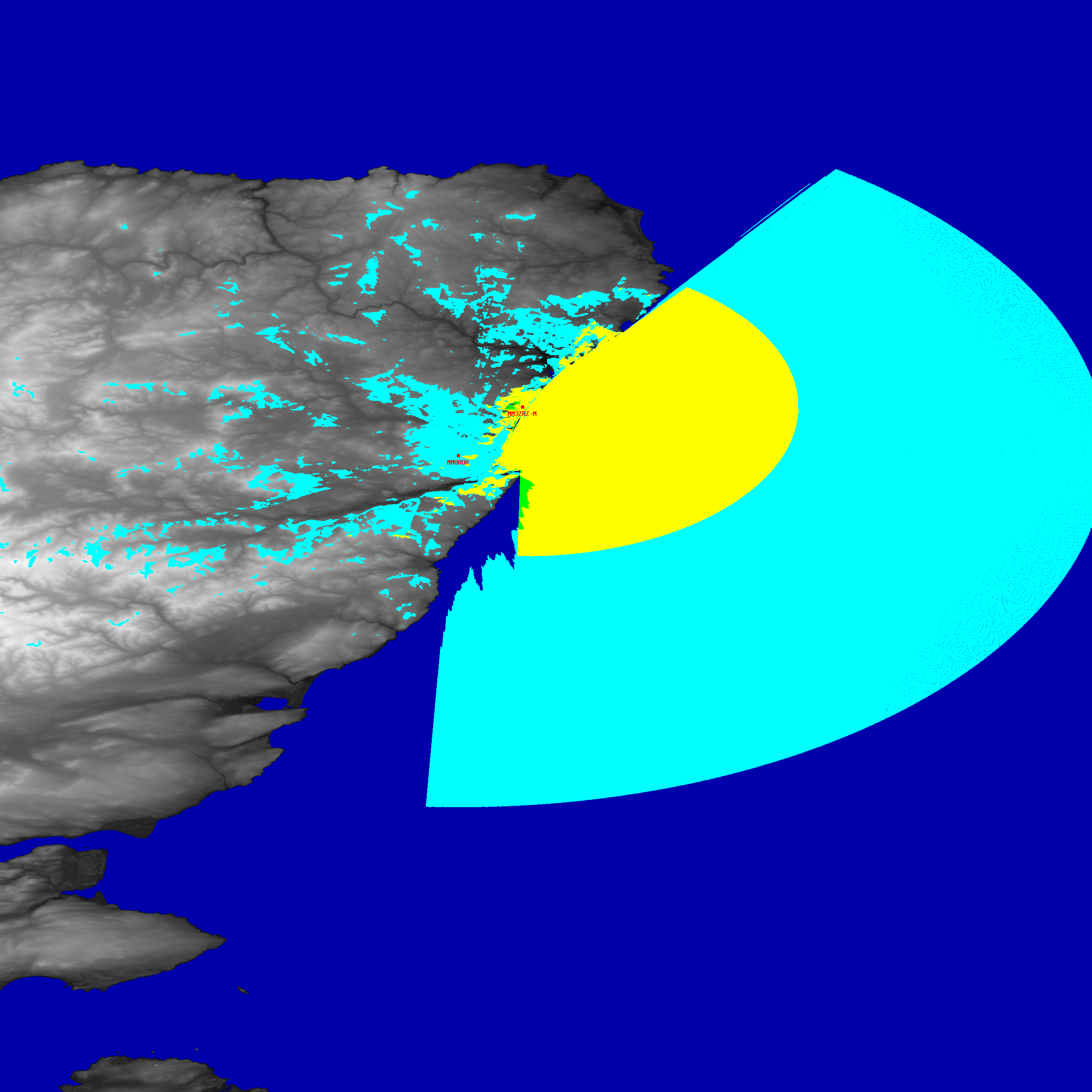
splat -t mm3zrz-m.qth mm0ror.qth -d ../sdf -c 20 -m 1.333 -o map-multiplayer.ppm

This outputs this image:

.

The splat man page has guidance for the colours, however the shortcut is:

The line-of-sight coverage is plotted in the following colours:

• MM3ZRZ-M: Green
• MM0ROR: Cyan
• Both: Yellow

We should be able to do a multiway net with someone at the beach and south south of the River Dee being able to hear us… kinda where Ed, MM6MVP lives, in fact (of course, his home location is obfuscated somewhat):

splat -t mm3zrz-m.qth mm0ror.qth -mm6mvp.qth d ../sdf -c 20 -m 1.333 -o map-triple.ppm

Outputting:

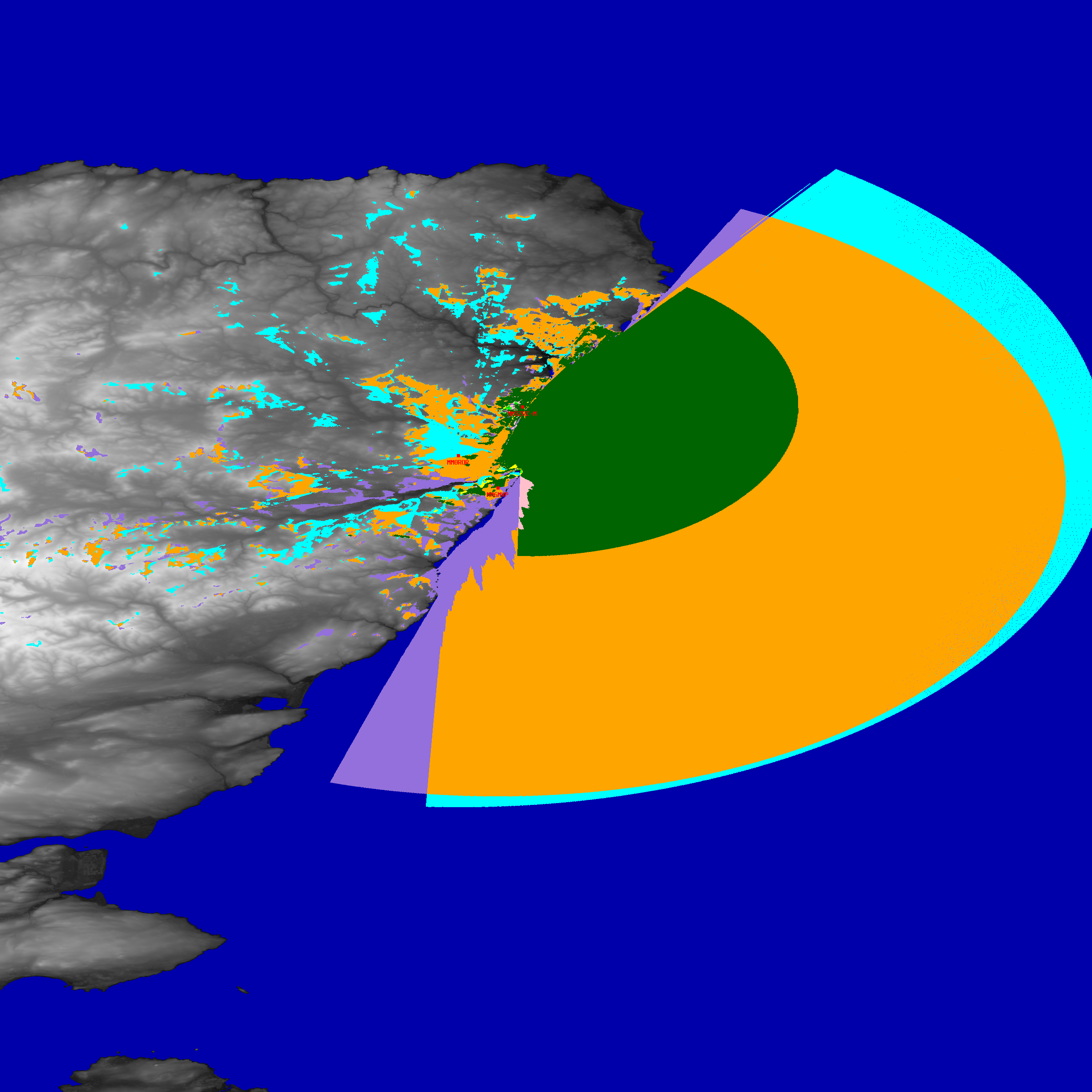
The line-of-sight coverage is plotted in the following colours:

• MM3ZRZ-M: Green
• MM0ROR: Cyan
• MM6MVP: Violet
• ZRZ&ROR: Yellow
• ZRZ&MVP: Pink
• ROR&MVP: Orange
• All 3: Dark Green

Yeah, maybe the 3 overlaid isn’t so clear…

Outcome

Once I learn more, I can see this being a really cool tool with lots of helpful features. Naturally, this is all simulated and the usual caveats apply - this is the best possible scenario, real life factors will make this perofrm worse and more.

I’m going to try and dig up more about antenna modelling in it, and start doing stuff like populating local towns and populated areas to make the map more busy and relatable.

Maybe I need to consider antenna modelling as a before and after and use this as a part of an entire link budget calculation.

It’ll be good to predict coverage with new bands, antennas and gear, and maybe plan some point-to-point fun with it.